# Import necessary libraries
import numpy as np
import matplotlib.pyplot as plt
import os1 Introduction
In my experience, many students and researchers invest significant effort into producing high-quality scientific work. However, when it comes to presenting their results, whether in journal papers, conference talks, or posters, the figures often fall short. Low-resolution images, inconsistent formatting, and cluttered visuals can take away from otherwise excellent work.
We put a lot of thought into how we present ourselves during seminars, conferences, or thesis defenses. The same level of care should go into how we present our visual materials. Figures are not just decorative, they are essential tools for communicating complex ideas clearly and effectively. In many cases, they are one of the first things readers look at in a paper or presentation.
This post shares practical tips for creating publication-ready scientific figures using Matplotlib in Python. While the focus is on Matplotlib, many of the same principles apply to tools like MATLAB or even Excel, although it is best to avoid Excel for final figures.
These days, there are many wrappers, GitHub projects, and blog posts built around Matplotlib that offer ready-made themes and color palettes. While these can be helpful starting points, there are a few core elements that still require your attention, such as figure format, font selection, legend placement, and overall clarity. Even if you are using Matplotlib’s default settings, small adjustments can make a big difference in the polish and professionalism of your figures.
Of course, it is fine to use rough plots early on to explore data or share quick results with your advisor. But those same plots should not be used in your final paper or presentation. If your research is strong, your visuals should reflect that. This guide will help you bring your figures up to the standard your work deserves.
2 Matplotlib Interfaces: pyplot versus axes
Matplotlib is a widely used, object-oriented plotting library offering two primary interfaces for creating figures: pyplot and axes. Knowing when to use each approach can be important for generating effective figures.
pyplot: Implicit (State-Based) Interface - This interface follows a MATLAB-like approach, where plotting functions operate on the current figure and axes behind the scenes. It is concise and convenient, making it ideal for quick visualizations or simple scripts, but it offers less control and flexibility.axes: Explicit (Object-Oriented) Interface - This interface provides fine-grained control over figures and axes by working directly with figure and axes objects. It is recommended for more complex figures, such as multi-panel figures or customized layouts.
The distinction between these interfaces can be initially confusing, especially when examples online mix both approaches. As a general guideline, the explicit object-oriented interface is better for multiple or intricate figures, while the implicit pyplot interface works well for simpler, single-subplot use cases.
Despite the differences, pyplot is almost always imported, regardless of which interface is chosen. This is because pyplot includes convenient utility functions that are essentially wrappers for axes methods, aiding in figure creation and management. Functions like pyplot.figure, pyplot.subplot, pyplot.subplots, and pyplot.savefig simplify common tasks and often serve as useful starting points.
This tutorial focuses only on the pyplot implicit interface, using a single subplot within a figure as the main example. The last section explains how to create multiple subplots within a single figure. For more details, you can refer to the official pyplot tutorial.
3 pyplot Implicit Interface
The first step is to import the necessary libraries. We will use NumPy and Matplotlib for this illustration, and will import more libraries as needed. Note that pyplot is imported as plt, so do not confuse it with plot, which is one of the functions within pyplot.
To illustrate, let’s plot the sine and cosine functions, with the data generated as follows.
# Generate data for sine and cosine functions
x = np.linspace(0, 20, 200)  # Generate 200 values between 0 and 20
y_sin = np.sin(x)  # Compute sine values
y_cos = np.cos(x)  # Compute cosine values
Here is how a Matplotlib figure looks with all the default settings. We will examine these settings later. Since we will use these plt commands multiple times, I have defined a function called sincos_plot() to simplify the process. We will update this function as we add more commands.
# Define a function to plot sine and cosine functions
def sincos_plot(title):
    """
    Plots sine and cosine functions with labels, title, and legend.

    Args:
        title (str): Title of the plot.
    """
    plt.plot(x, y_sin, label='sin')  # Plot sine function with a label
    plt.plot(x, y_cos, label='cos')  # Plot cosine function with a label
    plt.xlabel("Time (s)")  # Label for the x-axis
    plt.ylabel("Amplitude (m)")  # Label for the y-axis
    plt.title(title)  # Set the title of the plot
    plt.legend()  # Display the legend
    plt.show()  # Show the plot

# Call the function to plot with default options
sincos_plot(title='Default Options')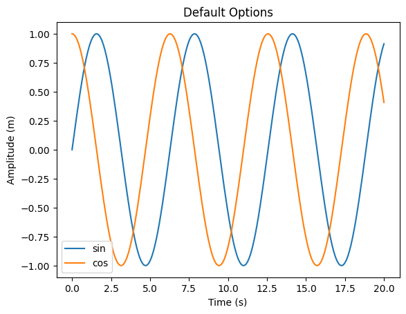
What are the issues with this figure? It looks pixelated because most of us save it in JPG or PNG format, which I will discuss further later on. The fonts appear unappealing compared to the rest of the document. Additionally, the aspect ratio (figure height vs. width) and legend location can be improved. This is just a simple figure, but take a look at some of the figures you have previously generated and see if you can identify some of these issues. Now, let us explore various ways to improve the figure.
3.1 Improvements
The Matplotlib library offers features to modify the appearance of each component of a figure. These features include options for altering the background, adding and customizing grids, adjusting the placement and appearance of titles, ticks, and text, as well as setting fonts for various graph elements, among other things. However, due to the vast number of parameters, configuring all of them can be a challenging task. We will focus on key areas: figure size and output format, font type, font and plot sizes, legend, axes frame, ticks, and grid. Before making modifications, consider reviewing the anatomy of a Matplotlib figure, which will guide us in customizing various elements in the following sections.
In Matplotlib, a figure is the overall container for a plot. It includes everything you see, such as one or more plots, titles, and labels. Axes (different from axis) refer to the actual plots inside the figure where data is drawn, and each Axes can have its own set of properties, such as x- and y-axis, title, labels, and limits.
One common analogy you see on the web explaining these two is that a figure is like a canvas, while axes are like individual paintings on that canvas. A figure can contain none or multiple axes (such as in subplots).
Note: This figure was created using Matplotlib and later edited with Affinity Designer.

Each time Matplotlib loads, whether you use the pyplot or axes interface, it defines a runtime configuration (rc) with default values for every figure element. This configuration can be adjusted by changing the values in rcParams, a dictionary that holds default values for various figure elements such as colors, fonts, line styles, and figure sizes. rcParams provides a way to set global styling preferences, ensuring consistent and visually appealing figures across multiple visualizations within a script or notebook. Changes to rcParams remain in effect throughout the Matplotlib session (or notebook) unless explicitly reset. To restore default values, you can use rcParams.update(matplotlib.rcParamsDefault). There are many ways to change the default values, as detailed in the official documentation.
Most of these elements can also be changed using pyplot functions. Essentially, pyplot modifies the rcParams in the backend. In the upcoming sections, we will adjust the rcParams parameters for each component, as we want most of these settings to be applied globally. I will also provide the final code on how to change these parameters using pyplot functions.
3.2 Figure Size and Output Format
3.2.1 Figure width and height
When creating high-quality figures, one of the first considerations should be the figure size and output format. A common mistake is setting the figure width too large for multiple subplots or too small for simpler plots. While these sizes may look fine in your plotting environment, problems often arise when figures are inserted into documents. They typically need to be scaled up or down to match the text width, which can distort font sizes and make labels, legends, and other elements difficult to read.
The default width and height of a Matplotlib figure are [6.4, 4.8] inches. There is no universal rule for selecting the figure’s dimensions, as the ideal size depends on the type of figure you are generating. However, here are some practical guidelines to help you make the right choices.
For technical reports in a single-column format, letter-size paper (8.5 × 11 inches) with 1-inch margins on both sides results in a usable text width of 6.5 inches. If you want a figure to span the full width of the text, setting the figure width to 6.5 inches is a good starting point. You can apply the same logic to other templates or formats by checking their text width and adjusting your figure accordingly. It is best to define the correct width directly when generating the figure in Matplotlib, rather than significantly scaling it down later.
To define the height, it is common practice to use an aspect ratio. Most figures are wider than they are tall, which is generally more visually appealing, especially for plots like time series or comparative bar charts. Modern screens and presentation formats often favor a 16:9 ratio over the older 4:3 format used in earlier templates. You can experiment with different ratios depending on the content and layout of your figure. In some cases, the height can exceed the width.
For simpler figures, using less than the full text width can maintain a clean and visually balanced layout. For example, the text width of this blog page is approximately 8.33 inches, but using 6.5 inches provides consistency and readability. For more complex figures, such as those with multiple subplots or intended for two-column templates, using the full width helps ensure that all elements remain clear and legible.
# Adjust figure size and re-plot
plt.figure(figsize=(15, 15 * 9 / 16))

sincos_plot(title='Scaling down the figure width of 15 inch')

# The `rcParams` for figure size will be applied to the next figure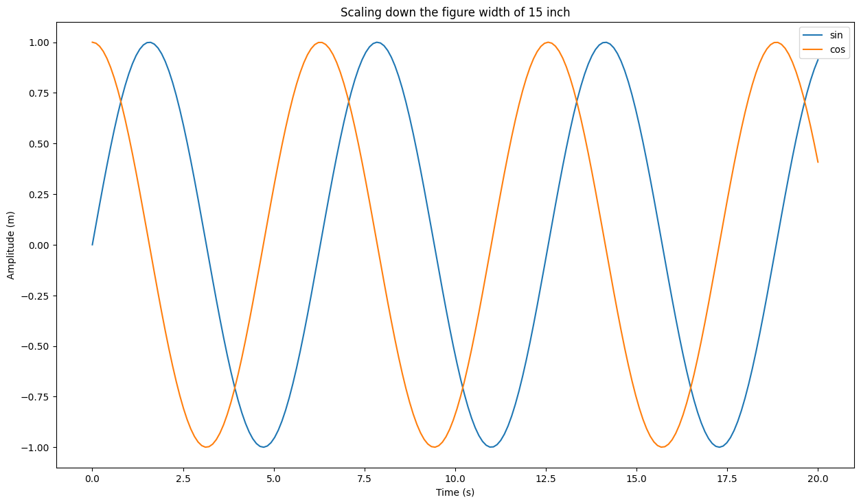
# Set figure size parameters
plt_width = (8.5 - 2 * 1) * 1
aspect_ratio = 0.4
plt_height = plt_width * aspect_ratio

# Apply figure size to rcParams
from matplotlib import rcParams
rcParams['figure.figsize'] = (plt_width, plt_height)

sincos_plot(title='Figure width = 6.5 inch')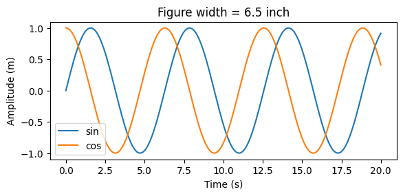
3.2.2 Output format and save options
When saving figures, choosing the appropriate file format based on the figure’s intended use is crucial. Image formats can be broadly categorized into raster and vector types.
Raster images store data as a grid of pixels, making them resolution-dependent. Common raster formats include PNG, JPEG, and TIFF. The default resolution in Matplotlib is 100 DPI, but most journals require a minimum of 300 DPI. Higher DPI values generally produce sharper images, but raster formats are not ideal for resizing. Enlarging a raster image can lead to pixelation or blurriness.
Vector images represent graphical elements as mathematical paths, making them resolution-independent. Common vector formats include SVG, PDF, and EPS. These are highly recommended for scientific publications because they scale cleanly, maintain sharpness at any size, and provide a professional-quality appearance. However, if your figure includes a large number of data points, vector rendering may become slow or problematic. In such cases, a high-DPI PNG is a good alternative. This blog post offers many great tips for getting the most precise text and images for publication.
If you are using LaTeX for document or presentation preparation, save your figures in PDF format. For PowerPoint, which is commonly used for presentations, save your figures in SVG format if you are on Windows, as these can be easily imported into PowerPoint or Word. If you are using macOS, you can paste PDF files directly into PowerPoint without any loss of quality, which simplifies the process.
Always save your figures using pyplot’s savefig() function, rather than saving manually from the output window. This ensures that all your figure settings, such as size, resolution, and layout adjustments, are preserved. The updated sincos_plot_save() function will include this saving capability, allowing you to specify the filename and desired file format.
By default, savefig() adds extra white space around the figure, and sometimes labels or titles may get clipped. A commonly used solution is bbox='tight', which removes extra padding, but this can shrink the overall figure size. A better approach is to enable figure.constrained_layout.use, which automatically adjusts spacing to ensure elements are well positioned and nothing gets cut off, without altering the intended figure dimensions.
# Update DPI and savefig parameters
rcParams['savefig.dpi'] = 300  # High resolution for saving figures
rcParams['savefig.bbox'] = 'tight'  # Remove extra padding when saving figures

# Create a directory for saving figures
savepath = 'figures'
os.makedirs(savepath, exist_ok=True)

# Define a function to save sine and cosine plots
def sincos_plot_save(title, fname):
    """
    Plots and saves sine and cosine functions with labels, title, and legend.

    Args:
        title (str): Title of the plot.
        fname (str): Filename to save the plot.
    """
    plt.figure()
    plt.plot(x, y_sin, label='sin')
    plt.plot(x, y_cos, label='cos')
    plt.xlabel("Time (s)")
    plt.ylabel("Amplitude (m)")
    plt.title(title)
    plt.legend()
    plt.savefig(os.path.join(savepath, fname))  # Save the plot
    plt.show()

# Save the vector plot in PDF format (for the web version SVG is used)
sincos_plot_save(title='Vector format, bbox = tight', fname='sincos_bbox.pdf')
rcParams['savefig.bbox'] = None # Reset
rcParams['figure.constrained_layout.use'] = True

sincos_plot_save(title='Vector format, constrained_layout', fname='sincos_constrained.pdf')
The figure included here is a raster image but still looks better because it uses 300 dpi. However, if you zoom in, the pixelation problem appears. Moreover, when we copy raster images into Word or PowerPoint or send them to a journal, programs can compress the figures, and they may look pixelated.
sincos_plot_save(title='Raster Format, DPI = 300', fname='sincos.png')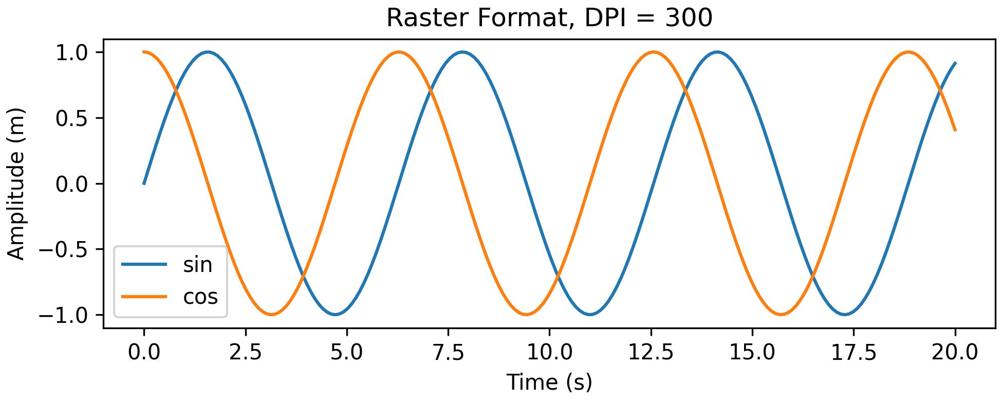
3.3 Font Type
For scientific writing, LaTeX is the preferred choice. Consequently, the best font to use for all graph elements in Matplotlib is Computer Modern, as it integrates seamlessly with the document and maintains a professional appearance. In MATLAB, using LaTeX rendering in figures is straightforward, but it is a bit trickier in Python. In this section, I’ll demonstrate how to use Computer Modern (cm) fonts included with Matplotlib, although this support is somewhat limited.
# Font settings: LaTeX-style
rcParams['font.family'] = 'serif'          # Set font family to serif
rcParams['font.serif'] = 'cmr10'           # Use Computer Modern Roman
rcParams['mathtext.fontset'] = 'cm'        # Use TeX-style math rendering
rcParams["axes.formatter.use_mathtext"] = True  # Properly render minus signs

sincos_plot_save(title='LaTeX font', fname='sincos_LaTeX.pdf')
While the figure above looks clean, vector figures rendered with an external LaTeX installation can appear dim on webpages, one of the main criticisms of using Computer Modern. However, it blends well in PDF documents. It is also possible to use other variants of the Computer Modern font that offer thicker or heavier weights.
For various reasons, LaTeX might not be an option. However, we can still choose a superior font family compared to the default Matplotlib font, which is DejaVu Sans. There are various font families and types available for use. Here are some Matplotlib core fonts that look good.
Check out this link to understand the differences between Serif and Sans Serif fonts, and use this link to see the fonts available on your machine.
# STIXGeneral font (available in matplotlib)
rcParams['font.family'] = 'serif'
rcParams['font.serif'] = 'STIXGeneral'

sincos_plot_save(title='STIXGeneral font', fname='sincos_STIX.pdf')

# Helvetica (sans-serif) font
# If the font is not available on your machine, the default sans-serif font will be used
# You can replace Helvetica with another sans-serif font available on your system such as Arial
rcParams['font.family'] = 'sans-serif'
rcParams['font.sans-serif'] = 'Helvetica'

sincos_plot_save(title='Helvetica font', fname='sincos_Helvetica.pdf')

Now that we have discussed figure size and font options, let’s explore how to manipulate various graph elements such as font sizes, widths, legend position, axes frame, grid and tick parameters (major, minor, width, direction), and color.
3.4 Font Size
Font size is crucial for ensuring that your data is readable and consistent with the rest of your document. Selecting the right font size for axis labels, tick marks, titles, and annotations can make the difference between a clear, effective figure and one that appears too cramped or overly large when included in a document.
A good rule of thumb is to keep figure text sizes close to the document’s body text size or slightly smaller. For example, if your paper uses 12-point body text, your figure labels should typically be in the 9–11 pt range. This ensures readability when the figure is inserted into a document or printed.
Here are some recommendations for font sizes:
| Element | Recommendation |
|---|---|
| Axis Labels and Legends | 10–11 pt; Match body text size for readability without zooming in |
| Tick Labels | 9–10 pt; Can be slightly smaller but should remain legible when scaled down |
| Annotations or Text | 9–11 pt; Same as axis labels or slightly smaller, based on importance |
| Title (within the figure) | 12–13 pt; Use for emphasis if needed, though titles are often better placed in captions |
Matplotlib follows a similar approach by automatically adjusting font sizes for various components of a figure. The default font size is 10 points, with other sizes primarily categorized as small, medium, and large, corresponding to scale factors of 0.833, 1, and 1.2, respectively. Specifically, axis labels and legend text use the medium font size (10 pt), titles are set to large (12 pt), and x and y tick labels also use the medium size (10 pt). If a new default font size is set, all text elements are proportionally scaled. There are many other categories available. It is better to set font sizes individually for each component. In this example, the font sizes of figures on the webpage are adjusted to correspond with the text size of the webpage, which is approximately 12 pt.
# Reset back to LaTeX-style serif font
rcParams['font.family'] = 'serif'
rcParams['font.serif'] = 'cmr10'
rcParams['mathtext.fontset'] = 'cm'
rcParams["axes.formatter.use_mathtext"] = True

# Set font sizes
rcParams['axes.labelsize'] = 11     # font size of x and y labels
rcParams['axes.labelpad'] = 5       # space between label and axis (default is 4)

rcParams['legend.fontsize'] = 11    # font size of legend

rcParams['xtick.labelsize'] = 10    # font size of xticks labels
rcParams['ytick.labelsize'] = 10    # font size of yticks labels

rcParams['axes.titlesize'] = 12     # font size of title

sincos_plot('Font Size')
3.5 Plot size/width
In addition to font sizes, line plot widths (or marker sizes in scatter plots) play a crucial role in the readability and visual balance of scientific figures. In Matplotlib, the default line width is set to 1.5, which works well for plots with a single data series. However, when a figure contains multiple lines, especially in comparative plots with several legends, it’s often better to use thinner lines (e.g., 0.75 to 1.25) to prevent visual clutter and overlapping. This approach helps maintain clarity and makes it easier for the reader to distinguish between different datasets.
For dense visualizations like spaghetti plots, where many time series or scenarios are shown together, it’s advisable to use very thin lines (e.g., 0.5 or less) for most of the data, while highlighting key lines, such as the mean or a reference scenario, with thicker widths (e.g., 1.5 to 2). This creates a natural visual hierarchy, guiding the reader’s attention to the most important information. Be sure to adjust these values according to the plot type and assess how well they integrate into the overall visual composition.
# Line width for plots
rcParams['lines.linewidth'] = 1

sincos_plot('Line Width')
3.6 Legend
Legends help readers understand what each line or marker in a figure represents. A well-placed, cleanly styled legend can improve clarity, while a poorly positioned one may overlap with data or clutter the figure. By default, Matplotlib uses loc='best' to place the legend in an area that avoids overlapping with figure elements. While this automatic placement can be helpful, it doesn’t always produce ideal results, especially when the data fills most of the plot area or when the figure’s width changes.
Matplotlib also offers standard positions like ‘upper right’, ‘lower left’, etc., which work well when there’s unused space, such as when the data doesn’t span the entire y-axis. However, in more complex plots with overlapping lines or many datasets (e.g., spaghetti plots), even corner placements can interfere with the visual content.
In such cases, it’s often better to move the legend outside the axes frame. If you are not using a title, placing the legend in a column format above the plot is also an option. To gain full control over legend positioning, especially outside the plot area, use the bbox_to_anchor argument with loc. This allows you to precisely position the legend relative to the axes.
Here are some recommendations for legends:
| Element | Recommendation |
|---|---|
| Location | Avoid overlap; place outside if needed using bbox_to_anchor |
| Entries | Use fewer legend entries when possible; highlight only key lines or groups |
| Font | Adjust font size to match or be slightly smaller than axis labels |
| Box | Use only if it helps separate the legend from a dense background; consider using transparency |
# Font size has already been adjusted in the font size section

# Remove legend frame
rcParams['legend.frameon'] = False

sincos_plot('Frame off')
3.6.1 bbox_to_anchor Options
You cannot directly set bbox_to_anchor through rcParams, as it is specific to individual legend placement logic at the figure or axes level. By default, bbox_to_anchor uses the axes coordinate system, where (0, 0) represents the lower-left corner and (1, 1) represents the upper-right corner of the axes. For example, setting bbox_to_anchor=(1, 1) with loc='upper right' positions the legend’s upper right corner at the top-right corner (1, 1) of the axes. In the figure below, the legend box is not exactly at the frame level due to default padding values. You can adjust these using the legend.borderaxespad option.
For more discussion on how to use bbox_to_anchor with legend locations, check out this link.
# rcParams['legend.loc'] = 'upper left' # legend location w.r.t bbox
# rcParams['legend.frameon'] = True   # change it to false if needed

# Plot with legend outside the figure
def sincos_plot_right(title):
    plt.plot(x, y_sin, label='sin')
    plt.plot(x, y_cos, label='cos')
    plt.xlabel("Time (s)")
    plt.ylabel("Amplitude (m)")
    plt.title(title)
    plt.legend(loc='upper left', bbox_to_anchor=(1, 1), frameon=True)
    plt.show()

sincos_plot_right('bbox to anchor')
Let’s position the legend where the title is and disable the title.
# rcParams['legend.loc'] = 'lower center' # legend location
# rcParams['legend.frameon'] = False   # change it to true if needed

# Legend positioned in place of the title
def sincos_plot_middle():
    plt.plot(x, y_sin, label='sin')
    plt.plot(x, y_cos, label='cos')
    plt.xlabel("Time (s)")
    plt.ylabel("Amplitude (m)")
    # plt.title(title)     # disable title
    # change legend to column format
    plt.legend(ncol=2, loc='lower center', bbox_to_anchor=(0.5, 0.95), frameon=False)
    plt.show()

sincos_plot_middle()
3.7 Axes Frame, Ticks, and Grid
Beyond font types, sizes, line widths, and legend position, a few subtle yet critical visual elements include deciding whether to display the axes frame (spines), the use of grid lines, and configuring major and minor ticks. These elements contribute significantly to making figures more readable.
Matplotlib applies a 5% margin around the data to provide visual padding. While some users prefer to remove these margins entirely for a tighter fit, it is generally better to retain them, especially when using inside ticks; the extra space ensures tick marks remain clearly visible. Adding a bit more margin along the y-axis can also improve the overall readability of the figure by preventing labels or data points from appearing too close to the edges. You can adjust these margin options based on the style you adopt.
3.7.1 Axes Frame (Spines)
By default, Matplotlib draws a full box around the plot using four spines (top, right, bottom, and left). For scientific plots, minimalist designs are often preferred. Removing the top and right spines reduces visual clutter while maintaining enough structure and directing attention to the data, rather than to the borders. Keeping all spines is common in many research papers, as it is the default option in many tools. Additionally, if subplots are used in the figure, the frame helps to visually separate them. If you choose to keep all spines, you can make them less prominent by reducing the frame width and using a shade of gray.
# Turn off right and top spines
rcParams['axes.spines.right'] = False
rcParams['axes.spines.top'] = False

# Customize axes options
rcParams['axes.linewidth'] = 0.6   # line width of axes bounding box (default = 0.8)
rcParams['axes.edgecolor'] = '0.20' # dark gray
rcParams['axes.xmargin'] = 0.02 # set x margin to 2%
rcParams['axes.ymargin'] = 0.10 # set y margin to 10%

# x and y tick styling
rcParams['xtick.direction'] = 'in'  # default = out
rcParams['xtick.major.size'] = 4    # default = 3.5
rcParams['xtick.major.width'] = 0.7 # default = 0.8

rcParams['ytick.direction'] = 'in'
rcParams['ytick.major.size'] = 4
rcParams['ytick.major.width'] = 0.7

sincos_plot_middle()
3.7.2 Grid Lines: To Use or Not?
Grid lines can be helpful for interpreting data values at a glance. However, in many cases, grid lines are avoided to reduce clutter. If you choose to use them, opt for light gray, dashed, or low-opacity grid lines to ensure they don’t overpower the data. Styles such as Seaborn’s darkgrid or ggplot, which use a gray background with white grid lines, are also commonly utilized, especially in the statistical field. These styles help maintain clarity while providing a structured background for the data.
# Turn top/right spines back on
rcParams['axes.spines.right'] = True
rcParams['axes.spines.top'] = True

# Enable grid
rcParams['axes.grid'] = True
rcParams['axes.grid.axis'] = 'both'
rcParams['grid.linewidth'] = 0.1    # default = 0.8
# custom line style: 50 pt dash, a 40 pt space, a 50 pt dash, and another 40 pt space, and then the sequence repeats
rcParams['grid.linestyle'] = [50, 40, 50, 40]   # default = -
rcParams['grid.color'] = '0.4'     # default = black

sincos_plot_right('Grid')
3.7.3 Tick Marks: Major and Minor
Ticks are essential guides that help readers interpret the scale and values of your plot. Their appearance in terms of length, thickness, and especially direction can influence the readability of a figure. Major ticks indicate the primary divisions on each axis and are typically longer and thicker. Minor ticks offer finer granularity and are usually shorter and lighter; they are helpful in log-scale plots or when high precision is required. Avoid overcrowding the axes with too many ticks, as this can reduce readability. Scientific publications typically favor ‘in’ ticks, especially when top and right spines are removed. If the figure will be embedded in a complex layout (e.g., with surrounding text, annotations, or subplots), ‘out’ ticks may be appropriate to avoid overlap.
# Disable grid
rcParams['axes.grid'] = False

# Minor ticks and extra styling
rcParams['xtick.top'] = True        # default = False
rcParams['xtick.direction'] = 'in'  # default = out
rcParams['xtick.major.size'] = 4    # default = 3.5
rcParams['xtick.major.width'] = 0.7 # default = 0.8
rcParams['xtick.minor.visible'] = True  # default = False
rcParams['xtick.minor.size'] = 2    # default = 2
rcParams['xtick.minor.width'] = 0.5 # default = 0.6

rcParams['ytick.right'] = True
rcParams['ytick.direction'] = 'in'
rcParams['ytick.major.size'] = 4
rcParams['ytick.major.width'] = 0.7
rcParams['ytick.minor.visible'] = True
rcParams['ytick.minor.size'] = 2
rcParams['ytick.minor.width'] = 0.5

sincos_plot_right('Ticks')
3.8 Color
Using color effectively, especially in scientific figures, requires more thought than simply relying on Matplotlib’s default color cycle, as color is a powerful tool in data visualization. While Matplotlib’s default colors are generally vibrant and distinct, they can become problematic when too many lines are plotted, the figure is printed in black and white, or when readers have color vision deficiencies. Although I won’t delve into the details of color theory, I recommend exploring articles and videos on this subject, as they often cover considerations for colorblind-friendly palettes and advice on avoiding certain color combinations, such as jet and rainbow color maps. When selecting color schemes, it’s useful to think in terms of the type of data you are visualizing. Here are three common categories:
| Data Type | Recommendation |
|---|---|
| Qualitative | For categorical or unordered data; use a palette of visually distinct, equally weighted colors without implying order (e.g., groups, categories, labels). |
| Sequential | For data with a natural order (low to high); use gradients that move from light to dark or shift through a single hue (e.g., heatmaps, contour plots, density plots). |
| Diverging | For data centered around a reference point (e.g., zero or average); use two contrasting colors that meet at a neutral center to show variation in both directions (e.g., residuals, difference maps). |
Classic color combinations like orange and blue or red and green (with adjusted saturation and lightness to make them colorblind-friendly) are often used for qualitative comparisons. However, it’s best to avoid highly saturated or overly bright colors, especially yellow or cyan, as they can appear harsh and are difficult to read against white backgrounds.
As a rule of thumb, try to limit the number of colors in a single figure to four or five. In many cases, high-quality figures can be created using only grayscale, combined with different line styles or marker shapes for distinction. In certain cases, color can be used to highlight important results, while the remaining elements can be in grayscale. When it comes to choosing color palettes, there are many resources and recommendations available. You can also create your own color palette with the help of these resources.
Principles of Beautiful Figures for Research Papers (watch the full video; highly recommended)
Paul Tol Color Scheme (color-blind safe palettes; Hex codes)
Your friendly guide to colors in data visualisation
Best Color Palettes for Scientific Figures and Data Visualizations
Choosing Colormaps in Matplotlib
Choosing Seaborn color palettes
# Change color cycle using axes.prop_cycle parameter
# Set custom color cycle: Paul Tol's vibrant color palette
# All six colors are displayed in the following three color figures
from cycler import cycler
rcParams['axes.prop_cycle'] = (cycler('color', ["#33BBEE", "#EE3377", "#0077BB", "#EE7733", "#CC3311", "#009988"]))

sincos_plot_right('Color')
# Use grayscale color and linestyle cycle
# 0 - black; 0.3 - dark gray; 0.5 - medium gray; 0.7 - light gray; 0.85 - very light gray
# - solid; -- dashed; -. dash dot; : dotted; 0, (3, 5, 1, 5) custom dash pattern
rcParams['axes.prop_cycle'] = (cycler('color', ['0.00', '0.30', '0.50', '0.70', '0.85']) +
                               cycler('linestyle', ['-', '--', '-.', ':', (0, (3, 5, 1, 5))]))

# Reduce clutter
rcParams['xtick.minor.visible'] = False
rcParams['ytick.minor.visible'] = False

sincos_plot_right('Grayscale')
3.9 pyplot complete code
What we have done so far can also be achieved using pyplot functions. The code below is a complete example of how to create a simple figure using pyplot with all the discussed features.
# Reset and rebuild final figure using pyplot
import numpy as np
import matplotlib.pyplot as plt

# Generate x values and corresponding sine and cosine values
x = np.linspace(0, 20, 200)
y_sin = np.sin(x)
y_cos = np.cos(x)

# Reset Matplotlib configuration to default settings
plt.rcParams.update(plt.rcParamsDefault)

# Update font settings for LaTeX-style appearance
rcParams['font.family'] = 'serif'
rcParams['font.serif'] = 'cmr10'
rcParams['mathtext.fontset'] = 'cm'
rcParams["axes.formatter.use_mathtext"] = True

# Create a new figure with a custom aspect ratio (width, height)
plt.figure(figsize=(6.5, 6.5 * 0.4))

# Plot sine and cosine curves with customized styles
plt.plot(x, y_sin, label='sin', linewidth=1, color= "#CC3311")
plt.plot(x, y_cos, label='cos', linewidth=1, linestyle='--', color="#009988")

# Axis labels and title
plt.xlabel("Time (s)", fontsize=11, labelpad=5)
plt.ylabel("Amplitude (m)", fontsize=11, labelpad=5)
plt.title('pyplot', fontsize=12)

# Customize tick parameters
plt.tick_params(
    axis='both', labelsize=10, which='major',
    direction='in', top=True, right=True, length=4, width=0.75
)

# Enable and style minor ticks
plt.minorticks_on()
plt.tick_params(axis='both', which='minor', direction='in',
                top=True, right=True, length=2, width=0.5)

# Set margins around data for clarity
plt.margins(x=0.02, y=0.1)

# Add legend with custom location and font size
plt.legend(
    fontsize=11, loc='upper left',
    bbox_to_anchor=(1, 1), frameon=True
)

# Add text with LaTeX-style formatting
plt.text(2.5, 0.8, "$\\sin(x)$", fontsize=11)

# Display the plot
plt.show()
3.10 Matplotlib Styles
While the pyplot functions allow you to achieve most styling tasks, using stylesheets or matplotlibrc files can simplify the process compared to specifying parameters for each figure individually. Matplotlib offers a variety of built-in stylesheets that you can apply to your figures. These stylesheets are predefined collections of parameters that determine the appearance of various figure elements, such as colors, fonts, line styles, and more.
Additionally, you have the option to create your own custom stylesheets. For instance, you can develop one based on the parameters we have discussed. Custom stylesheets can be tailored for different templates, such as single-column, double-column, or PowerPoint formats. This flexibility allows you to easily switch styles depending on the context in which you are using the figures. When preparing a figure for a journal article, you might choose a style optimized for publication. Conversely, for a presentation, you may opt for a style that is visually appealing and easy to read on a screen.
To apply a style, use the plt.style.use() function and specify the name of the style you wish to use. For instance, to apply the ‘ggplot’ style, you would use: plt.style.use('ggplot'). You can also create custom styles by defining a .mplstyle file with your chosen parameters. To apply a custom style, simply provide the path to the .mplstyle file within the plt.style.use() function.
The .mplstyle file, based on the rcParams we discussed, is available in the Code Links section to the right. If you use bbox_to_anchor, it must be explicitly specified in the plt.legend function. You can adjust the parameters as needed.
3.10.1 Style sheets
Matplotlib style sheets reference
Science Plots (Matplotlib styles for scientific figures)
3.10.2 Popular Matplotlib wrappers
Seaborn (statistical data visualization)
UltraPlot (create publication-quality figures; formerly known as ProPlot)
plotnine (implementation of the grammar of graphics in Python, similar to ggplot2 in R)
# Load custom style
plt.style.use('default')    # Reset to default settings
plt.style.use('letter12.mplstyle')

plt.plot(x, y_sin, label='sin')
plt.plot(x, y_cos, label='cos')

plt.xlabel("Time (s)")
plt.ylabel("Amplitude (m)")
plt.title('letter12.mplstyle')
plt.legend(bbox_to_anchor=(1, 1))
plt.show()
3.11 Multiple Subplots
So far, we have focused on creating a single subplot using the pyplot implicit interface. However, in many cases, you may need to create multiple subplots within a single figure. This is especially common when comparing different datasets or visualizing multiple aspects of the same data. We can create multiple subplots using the plt.subplots() function. This function allows you to specify the number of rows and columns of subplots, as well as their size and layout.
plt.subplots(2, 1, figsize=(6.5, 6.5 * 0.75), sharex=True, gridspec_kw={'hspace': 0.1})
plt.subplot(211)    # same as plt.subplot(2, 1, 1)
plt.plot(x, y_sin, label='sin', color=f'C{0}')
# plt.xlabel("Time (s)")
plt.ylabel("Amplitude (m)")
plt.title('Sine plot')

plt.subplot(212)    # same as plt.subplot(2, 1, 2)
plt.plot(x, y_cos, label='cos', color=f'C{1}')
plt.xlabel("Time (s)")
plt.ylabel("Amplitude (m)")
plt.title('Cosine plot')
plt.show()
plt.subplots(1, 2, figsize=(7.5, 7.5 * 0.3), sharey=True)
# plt.get_layout_engine().set(w_pad=4 / 72, h_pad=4 / 72, hspace=0.2,
                            # wspace=0.2)
# plt.subplots_adjust(wspace=0.4)  # Adjust space between subplots
plt.subplot(121)
plt.plot(x, y_sin, label='sin', color=f'C{0}')
plt.xlabel("Time (s)")
plt.ylabel("Amplitude (m)")
plt.title('Sine plot')

plt.subplot(122)
plt.plot(x, y_cos, label='cos', color=f'C{1}')
plt.xlabel("Time (s)")
# plt.ylabel("Amplitude (m)")
plt.title('Cosine plot')
plt.show()